Assignment 3

---

Research Question

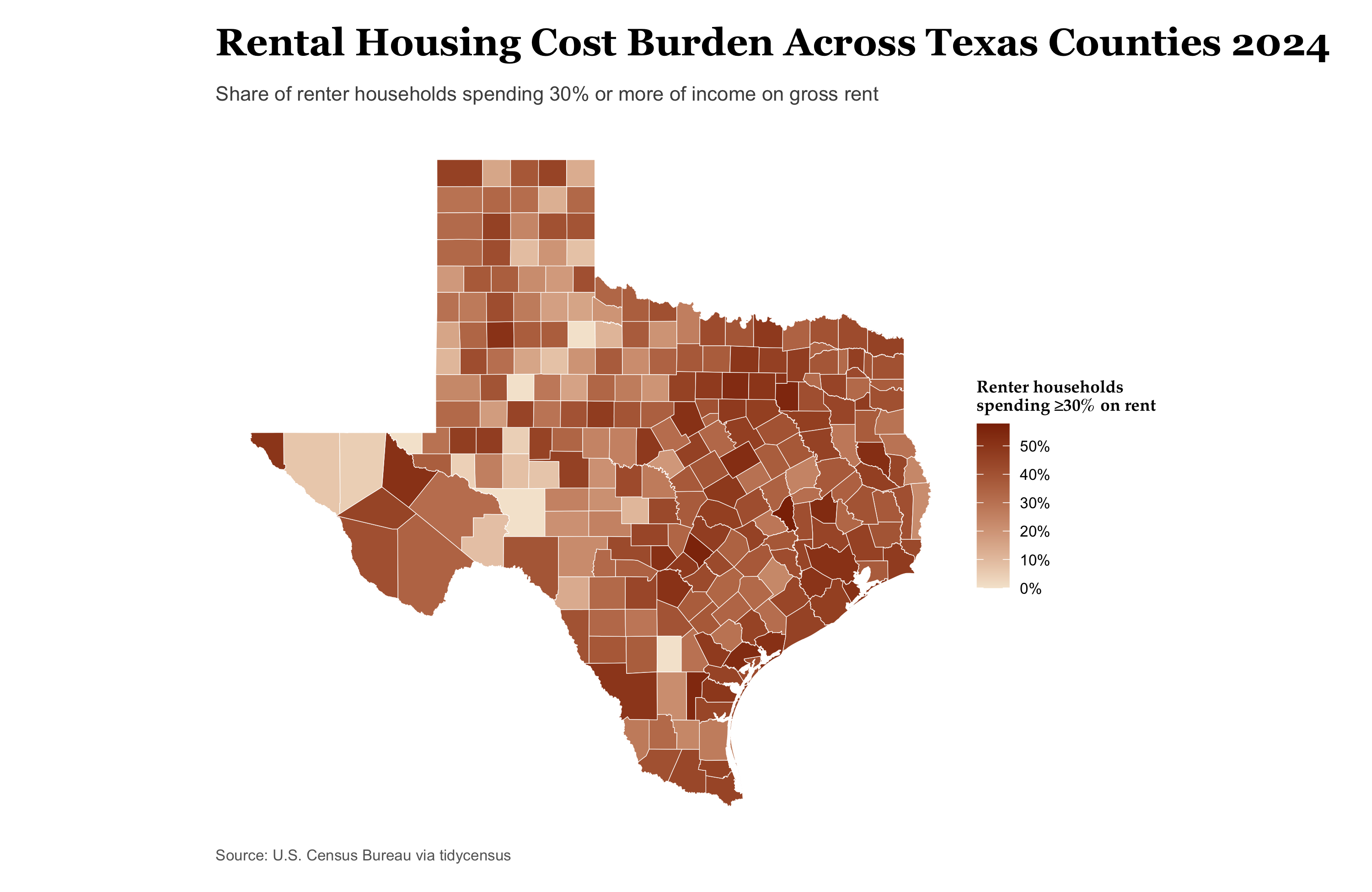
What is the distribution of rental housing cost burden across Texas counties?

I measure rental housing cost burden as the share of renter households that spend 30% or more of their household income on gross rent. I also examine median household income as a second measure of the socioeconomic conditions of each county.

1. Setup

# Packages

library(tidycensus)
library(tigris)

To enable caching of data, set `options(tigris_use_cache = TRUE)`
in your R script or .Rprofile.

library(sf)

Linking to GEOS 3.13.0, GDAL 3.8.5, PROJ 9.5.1; sf_use_s2() is TRUE

library(dplyr)

Attaching package: 'dplyr'

The following objects are masked from 'package:stats':

    filter, lag

The following objects are masked from 'package:base':

    intersect, setdiff, setequal, union

library(tidyr)
library(ggplot2)
library(readr)

options(tigris_use_cache = TRUE)

# Explore variables 

vars <- load_variables(2024, "acs5")

vars |>
  filter(name %in% c(
    "B25070_001",
    "B25070_007",
    "B25070_008",
    "B25070_009",
    "B25070_010",
    "B19013_001"
  ))

# A tibble: 6 × 4
  name       label                                             concept geography
  <chr>      <chr>                                             <chr>   <chr>    
1 B19013_001 Estimate!!Median household income in the past 12… Median… block gr…
2 B25070_001 Estimate!!Total:                                  Gross … block gr…
3 B25070_007 Estimate!!Total:!!30.0 to 34.9 percent            Gross … block gr…
4 B25070_008 Estimate!!Total:!!35.0 to 39.9 percent            Gross … block gr…
5 B25070_009 Estimate!!Total:!!40.0 to 49.9 percent            Gross … block gr…
6 B25070_010 Estimate!!Total:!!50.0 percent or more            Gross … block gr…

vars |>
  filter(grepl("^B25070", name))

# A tibble: 11 × 4
   name       label                                    concept         geography
   <chr>      <chr>                                    <chr>           <chr>    
 1 B25070_001 Estimate!!Total:                         Gross Rent as … block gr…
 2 B25070_002 Estimate!!Total:!!Less than 10.0 percent Gross Rent as … block gr…
 3 B25070_003 Estimate!!Total:!!10.0 to 14.9 percent   Gross Rent as … block gr…
 4 B25070_004 Estimate!!Total:!!15.0 to 19.9 percent   Gross Rent as … block gr…
 5 B25070_005 Estimate!!Total:!!20.0 to 24.9 percent   Gross Rent as … block gr…
 6 B25070_006 Estimate!!Total:!!25.0 to 29.9 percent   Gross Rent as … block gr…
 7 B25070_007 Estimate!!Total:!!30.0 to 34.9 percent   Gross Rent as … block gr…
 8 B25070_008 Estimate!!Total:!!35.0 to 39.9 percent   Gross Rent as … block gr…
 9 B25070_009 Estimate!!Total:!!40.0 to 49.9 percent   Gross Rent as … block gr…
10 B25070_010 Estimate!!Total:!!50.0 percent or more   Gross Rent as … block gr…
11 B25070_011 Estimate!!Total:!!Not computed           Gross Rent as … block gr…

vars |>
  filter(grepl("^B19013", name))

# A tibble: 10 × 4
   name        label                                           concept geography
   <chr>       <chr>                                           <chr>   <chr>    
 1 B19013A_001 Estimate!!Median household income in the past … Median… tract    
 2 B19013B_001 Estimate!!Median household income in the past … Median… tract    
 3 B19013C_001 Estimate!!Median household income in the past … Median… tract    
 4 B19013D_001 Estimate!!Median household income in the past … Median… tract    
 5 B19013E_001 Estimate!!Median household income in the past … Median… county   
 6 B19013F_001 Estimate!!Median household income in the past … Median… tract    
 7 B19013G_001 Estimate!!Median household income in the past … Median… tract    
 8 B19013H_001 Estimate!!Median household income in the past … Median… tract    
 9 B19013I_001 Estimate!!Median household income in the past … Median… tract    
10 B19013_001  Estimate!!Median household income in the past … Median… block gr…

2. Select Geography and Variables

I use Texas counties because county-level geography allows for a statewide comparison while keeping the map readable.

The ACS table B25070 provides the number of renter-occupied households by the percentage of income spent on gross rent. I combine the categories from 30% through 50% or more to create the numerator for the rent-burden rate.

I also use B19013, median household income, as a second variable.

# Parameters

state_abbr <- "TX"
geo_level <- "county"

my_vars <- c(
  renters = "B25070_001",
  burden_30_35 = "B25070_007",
  burden_35_40 = "B25070_008",
  burden_40_50 = "B25070_009",
  burden_50_plus = "B25070_010",
  income = "B19013_001"
)

year_acs <- 2024
survey <- "acs5"

3. Check the Variables

vars <- load_variables(2024, "acs5")

vars |>
  filter(name %in% c(
    "B25070_001",
    "B25070_007",
    "B25070_008",
    "B25070_009",
    "B25070_010",
    "B19013_001"
  ))

# A tibble: 6 × 4
  name       label                                             concept geography
  <chr>      <chr>                                             <chr>   <chr>    
1 B19013_001 Estimate!!Median household income in the past 12… Median… block gr…
2 B25070_001 Estimate!!Total:                                  Gross … block gr…
3 B25070_007 Estimate!!Total:!!30.0 to 34.9 percent            Gross … block gr…
4 B25070_008 Estimate!!Total:!!35.0 to 39.9 percent            Gross … block gr…
5 B25070_009 Estimate!!Total:!!40.0 to 49.9 percent            Gross … block gr…
6 B25070_010 Estimate!!Total:!!50.0 percent or more            Gross … block gr…

4. Download the ACS Data

I use the 2024 ACS 5-year estimates and keep the geometry so that the county-level data can be mapped.

# Download, wide — one row per area, and the sf class survives

acs_wide <- get_acs(
  geography = geo_level,
  variables = my_vars,
  state = state_abbr,
  year = year_acs,
  survey = survey,
  geometry = TRUE,
  output = "wide"
)

Getting data from the 2020-2024 5-year ACS

5. Create the Rent-Burden Numerator

The rent-burden numerator is the number of renter households spending 30% or more mof their income on gross rent. I combine the four relevant ACS categories.

# Derive a rate, and carry its margin of error through

acs_wide <- acs_wide |>
  mutate(
    burden_30_plusE =
      burden_30_35E +
      burden_35_40E +
      burden_40_50E +
      burden_50_plusE
  )

6. Calculate the Rent-Burden Rate

The denominator is the total number of renter-occupied households. I divide the number of households spending 30% or more of income on rent by the total number of renter households.

acs_wide <- acs_wide |>
  mutate(
    burden_rate = burden_30_plusE / rentersE
  )

I then convert the rate to a percentage for easier interpretation.

acs_wide <- acs_wide |>
  mutate(
    burden_pct = burden_rate * 100
  )

7. Carry the Margin of Error Through the Calculation

Because the numerator combines four ACS estimates, I first calculate its margin of error using moe_sum().

acs_wide <- acs_wide |>
  rowwise() |>
  mutate(
    burden_30_plusM = moe_sum(
      c(
        burden_30_35M,
        burden_35_40M,
        burden_40_50M,
        burden_50_plusM
      ),
      estimate = c(
        burden_30_35E,
        burden_35_40E,
        burden_40_50E,
        burden_50_plusE
      )
    )
  ) |>
  ungroup()

I then use moe_prop() to carry the uncertainty through the calculation of the rent-burden rate.

acs_wide <- acs_wide |>
  mutate(
    burden_moe = moe_prop(
      burden_30_plusE,
      rentersE,
      burden_30_plusM,
      rentersM
    ),
    burden_moe_pct = burden_moe * 100
  )

8. Check the Results

acs_wide |>
  select(
    NAME,
    burden_30_plusE,
    burden_30_plusM,
    rentersE,
    rentersM,
    burden_pct,
    burden_moe_pct
  ) |>
  slice_head(n = 10)

Simple feature collection with 10 features and 7 fields
Geometry type: MULTIPOLYGON
Dimension:     XY
Bounding box:  xmin: -105.998 ymin: 27.20931 xmax: -93.79455 ymax: 33.71599
Geodetic CRS:  NAD83
# A tibble: 10 × 8
   NAME             burden_30_plusE burden_30_plusM rentersE rentersM burden_pct
   <chr>                      <dbl>           <dbl>    <dbl>    <dbl>      <dbl>
 1 Lee County, Tex…             702           279.      1550      376      45.3 
 2 Bowie County, T…            5818           678.     12820      692      45.4 
 3 Kleberg County,…            2466           532.      5628      498      43.8 
 4 Hudspeth County…              15            21.2      222       79       6.76
 5 Shelby County, …             711           239.      2434      365      29.2 
 6 Loving County, …               0            15         24       28       0   
 7 Montgomery Coun…           31014          1974.     69884     2344      44.4 
 8 Bexar County, T…          156399          4103.    309018     3657      50.6 
 9 Jefferson Count…           16872          1257.     35551     1264      47.5 
10 Tyler County, T…             504           166.      1345      225      37.5 
# ℹ 2 more variables: burden_moe_pct <dbl>, geometry <MULTIPOLYGON [°]>

9. Map: Rental Housing Cost Burden

The map shows the share of renter households in each Texas county spending 30% or more of their income on gross rent.

rent_burden_map <- ggplot(acs_wide) +
  geom_sf(
    aes(fill = burden_pct),
    color = "white",
    linewidth = 0.15
  ) +
  scale_fill_gradient(
    low = "#F5E6D3",
    high = "#8C2D04",
    name = "Renter households\nspending ≥30% on rent",
    labels = function(x) paste0(x, "%")
  ) +
  labs(
    title = "Where Rent Takes Up More of Household Income",
    subtitle = "Share of renter households spending 30% or more of income on gross rent, Texas counties",
    caption = "Source: U.S. Census Bureau, 2024 ACS 5-year estimates"
  ) +
  theme_void() +
  theme(
    text = element_text(family = "Arial"),
    
    plot.title = element_text(
      family = "Georgia",
      size = 20,
      face = "bold",
      hjust = 0,
      margin = margin(b = 8)
    ),
    
    plot.subtitle = element_text(
      family = "Arial",
      size = 10.5,
      color = "gray30",
      hjust = 0,
      margin = margin(b = 12)
    ),
    
    legend.position = "right",
    
    legend.title = element_text(
      family = "Arial",
      size = 9,
      face = "bold"
    ),
    
    legend.text = element_text(
      family = "Arial",
      size = 8
    ),
    
    plot.caption = element_text(
      family = "Arial",
      size = 8,
      color = "gray40",
      hjust = 0
    ),
    
    plot.margin = margin(15, 15, 15, 15)
  )

10. Table

a) Highest-Income Counties

I rank counties by median household income and show the rent-burden estimate and its margin of error alongside income.

top10_income <- acs_wide |>
  st_drop_geometry() |>
  arrange(desc(incomeE)) |>
  select(
    NAME,
    incomeE,
    incomeM,
    burden_pct,
    burden_moe_pct
  ) |>
  slice_head(n = 10)

top10_income

# A tibble: 10 × 5
   NAME                     incomeE incomeM burden_pct burden_moe_pct
   <chr>                      <dbl>   <dbl>      <dbl>          <dbl>
 1 Rockwall County, Texas    127981    4257      50.7            6.43
 2 Collin County, Texas      121600    1883      45.8            1.53
 3 Kendall County, Texas     114962    8014      51.7            8.83
 4 Fort Bend County, Texas   114041    1899      50.2            2.85
 5 Denton County, Texas      111498    1485      49.5            1.63
 6 Williamson County, Texas  111340    1581      46.4            2.17
 7 Chambers County, Texas    109804   10467      37.0           10.2 
 8 Parker County, Texas      104443    3349      47.9            5.75
 9 Comal County, Texas       101889    2995      48.5            5.04
10 Glasscock County, Texas   101250   53302       4.14          11.5 

b) Lowest-Income Counties

bottom10_income <- acs_wide |>
  st_drop_geometry() |>
  arrange(incomeE) |>
  select(
    NAME,
    incomeE,
    incomeM,
    burden_pct,
    burden_moe_pct
  ) |>
  slice_head(n = 10)

bottom10_income

# A tibble: 10 × 5
   NAME                   incomeE incomeM burden_pct burden_moe_pct
   <chr>                    <dbl>   <dbl>      <dbl>          <dbl>
 1 Swisher County, Texas    36165   14512       36.1          13.0 
 2 Zavala County, Texas     36749    5834       33.0          13.1 
 3 Starr County, Texas      37639    4431       40.5           5.60
 4 Dimmit County, Texas     38808    8956       38.3          16.2 
 5 Kenedy County, Texas     38882    4589       26.9          69.6 
 6 Zapata County, Texas     39239    4265       27.4          12.5 
 7 Real County, Texas       39605   34535       32.4          18.7 
 8 Edwards County, Texas    40313   21695       22.4          37.3 
 9 Jim Hogg County, Texas   42211    3821       32.6          22.1 
10 Newton County, Texas     42618    5785       22.2           9.30

c) Complete Table

# 10) Table — top and bottom 10 counties by median household income

top10 <- acs_wide |>
  st_drop_geometry() |>
  arrange(desc(incomeE)) |>
  transmute(
    Group = "Top 10",
    County = NAME,
    `Median household income` = incomeE,
    `Income MOE` = incomeM,
    `Rent burden (%)` = burden_pct,
    `MOE (%)` = burden_moe_pct
  ) |>
  slice_head(n = 10)

bottom10 <- acs_wide |>
  st_drop_geometry() |>
  arrange(incomeE) |>
  transmute(
    Group = "Bottom 10",
    County = NAME,
    `Median household income` = incomeE,
    `Income MOE` = incomeM,
    `Rent burden (%)` = burden_pct,
    `MOE (%)` = burden_moe_pct
  ) |>
  slice_head(n = 10)

income_table <- bind_rows(top10, bottom10) |>
  mutate(
    `Median household income` =
      paste0("$", format(round(`Median household income`), big.mark = ",")),
    `Income MOE` =
      paste0("$", format(round(`Income MOE`), big.mark = ",")),
    `Rent burden (%)` =
      round(`Rent burden (%)`, 1),
    `MOE (%)` =
      round(`MOE (%)`, 1)
  )

knitr::kable(
  income_table,
  caption = "Top and Bottom 10 Texas Counties by Median Household Income",
  align = c("l", "l", "r", "r", "r", "r")
)

Top and Bottom 10 Texas Counties by Median Household Income

Group	County	Median household income	Income MOE	Rent burden (%)	MOE (%)
Top 10	Rockwall County, Texas	$127,981	$ 4,257	50.7	6.4
Top 10	Collin County, Texas	$121,600	$ 1,883	45.8	1.5
Top 10	Kendall County, Texas	$114,962	$ 8,014	51.7	8.8
Top 10	Fort Bend County, Texas	$114,041	$ 1,899	50.2	2.8
Top 10	Denton County, Texas	$111,498	$ 1,485	49.5	1.6
Top 10	Williamson County, Texas	$111,340	$ 1,581	46.4	2.2
Top 10	Chambers County, Texas	$109,804	$10,467	37.0	10.2
Top 10	Parker County, Texas	$104,443	$ 3,349	47.9	5.8
Top 10	Comal County, Texas	$101,889	$ 2,995	48.5	5.0
Top 10	Glasscock County, Texas	$101,250	$53,302	4.1	11.5
Bottom 10	Swisher County, Texas	$ 36,165	$14,512	36.1	13.0
Bottom 10	Zavala County, Texas	$ 36,749	$ 5,834	33.0	13.1
Bottom 10	Starr County, Texas	$ 37,639	$ 4,431	40.5	5.6
Bottom 10	Dimmit County, Texas	$ 38,808	$ 8,956	38.3	16.2
Bottom 10	Kenedy County, Texas	$ 38,882	$ 4,589	26.9	69.6
Bottom 10	Zapata County, Texas	$ 39,239	$ 4,265	27.4	12.5
Bottom 10	Real County, Texas	$ 39,605	$34,535	32.4	18.7
Bottom 10	Edwards County, Texas	$ 40,313	$21,695	22.4	37.3
Bottom 10	Jim Hogg County, Texas	$ 42,211	$ 3,821	32.6	22.1
Bottom 10	Newton County, Texas	$ 42,618	$ 5,785	22.2	9.3

12. Uncertainty Check

To examine uncertainty, I calculate an interval around each rent-burden estimate using its ACS margin of error. I then check whether the intervals for adjacent counties in the table overlap.

uncertainty_check <- top10_income |>
  mutate(
    lower = burden_pct - burden_moe_pct,
    upper = burden_pct + burden_moe_pct
  ) |>
  mutate(
    next_county = lead(NAME),
    next_lower = lead(lower),
    next_upper = lead(upper),
    overlap = lower <= next_upper & upper >= next_lower
  ) |>
  filter(overlap) |>
  slice_head(n = 1)

uncertainty_check

# A tibble: 1 × 11
  NAME         incomeE incomeM burden_pct burden_moe_pct lower upper next_county
  <chr>          <dbl>   <dbl>      <dbl>          <dbl> <dbl> <dbl> <chr>      
1 Rockwall Co…  127981    4257       50.7           6.43  44.2  57.1 Collin Cou…
# ℹ 3 more variables: next_lower <dbl>, next_upper <dbl>, overlap <lgl>

The code identifies Rockwall County and Collin County as a pair whose intervals overlap.

Rockwall County has an estimated rent-burden rate of 50.7%, with an interval from approximately 44.2% to 57.1%. Collin County has an estimated rate of 45.8%, with an interval from approximately 44.3% to 47.4%.

Because these intervals overlap, the difference between the two estimated rent-burden rates should be interpreted cautiously. The overlap does not change the ranking by median household income, but it shows that the difference in the accompanying rent-burden estimates is not clearly distinguishable given sampling uncertainty.

# Save outputs
write_csv(st_drop_geometry(acs_wide),
          paste0("acs_", state_abbr, "_", year_acs, ".csv"))

13. Methods

This analysis uses 2024 ACS 5-year estimates to examine rental housing cost burden across Texas counties. County-level geography was selected because it provides a statewide comparison while remaining readable on a choropleth map. Rental housing cost burden is measured as the share of renter-occupied households spending 30% or more of household income on gross rent. The numerator combines households spending 30–34.9%, 35–39.9%, 40–49.9%, and 50% or more of income on rent, while total renter-occupied households provide the denominator. Median household income is included as a second socioeconomic measure. Because ACS estimates are based on samples, each estimate has a margin of error. I calculate and report the MOE for the rent-burden rate rather than treating the estimates as exact values. Overlapping confidence intervals indicate that small differences between counties should not automatically be interpreted as meaningful differences in the estimates.